AMR & AGVs
How Many AMRs Do You Actually Need? A Guide to Throughput Modeling
Sep 24, 2026 · 15 min read · Robotech Pros
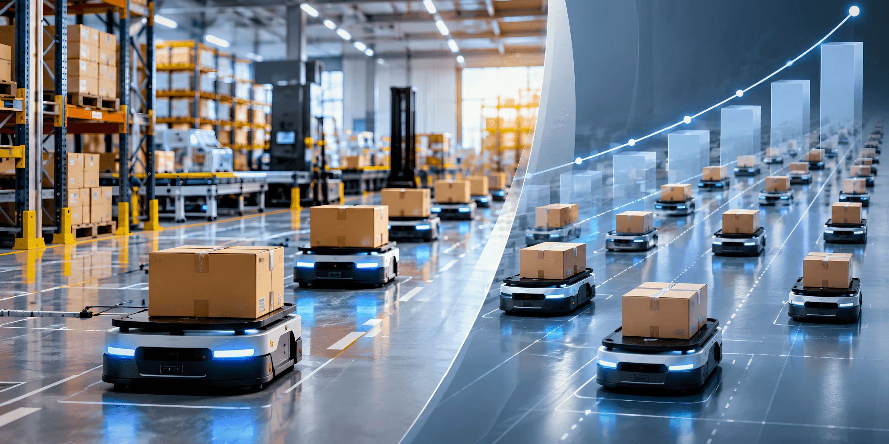
Most AMR fleet sizes are guessed before anyone counts the moves. This guide walks through the four-step throughput model that replaces the guess, and explains why doubling throughput takes more than double the robots.
How Many AMRs Do You Actually Need? A Guide to Throughput Modeling
Most fleet sizing conversations start with a number somebody already has in mind. Six robots. Twelve. Twenty. The figure usually arrives from a vendor demonstration, a peer facility, or a budget line, and it lands before anyone has written down how many moves the operation actually needs per hour.
That order of operations is expensive in both directions. Undersize the fleet and the pilot misses a throughput target it was never equipped to hit. Oversize it and you pay for robots that spend the shift queued behind each other in an aisle.
Throughput modeling is what replaces the guess. The math is not difficult. It is four steps, and the discipline is in refusing to skip any of them.
Why Dividing Demand by Speed Gives the Wrong Answer
The intuitive model is distance divided by speed, multiplied by the number of moves, divided by the hours in a shift. It produces a clean number, and the number is almost always too low. Two things break it.
The first is that a rated speed is a laboratory figure. A common 250 kg-class AMR has a rated maximum speed of 2.0 m/s, measured in controlled conditions. In a working aisle it slows for people, decelerates into turns, and spends time docking to within a few millimeters. Until you have measured your own routes, plan on roughly half the rated speed. At least one published sizing method assumes a travel speed of about 1 m/s.
The second is that robots interfere with one another. Fleet size and per-robot productivity are not independent variables. Research on fleet sizing using closed queueing network models states it directly: as the fleet grows, each vehicle completes fewer trips, and beyond a certain fleet size throughput rises only marginally while cycle time increases sharply. Research published by MIT with Symbotic in March 2026 points the same way: smarter traffic coordination delivered about 25 percent more throughput in warehouse simulations, and the researchers noted that conventional coordination methods start to break down as robot density rises. Density costs throughput, and the cost grows with scale.
An honest model therefore derates before it divides. The twentieth robot in an aisle does less work than the fifth.
Step 1. Define Demand at Peak, Not on Average
One of the most common errors in fleet sizing is dividing daily volume by shift hours and calling the result demand. Warehouses do not run flat. They run in waves shaped by carrier cutoffs, wave release, replenishment cycles and inbound schedules. Size to the hour that actually hurts: pull twelve months of transaction history, find the busiest hour of a normal busy day, then check what the peak week does to that figure.
Define the unit before you count anything. A move is one loaded leg from origin to destination. Whether a round trip counts as one move or two is a convention rather than a fact, so pick one and hold it through the entire model. And if you are still deciding whether product travels to the picker or the picker travels to product, that choice changes the move count more than any robot specification will. Our comparison of goods-to-person and person-to-goods models is the place to settle it.
Table 1: Inputs to a Defensible Demand Profile
| Input | Where the number comes from | Common error |
|---|---|---|
| Move definition | Process map, agreed before counting starts | Counting a round trip as one move in one place and two in another |
| Peak hour volume | WMS transaction history, busiest hour of a normal busy day | Dividing daily volume by shift hours |
| Seasonal peak factor | Peak week compared against an average week across 12 months | Sizing to the annual average and absorbing Q4 with overtime |
| Moves per order line | Process map including replenishment, putaway and returns | Counting outbound picks only |
| Hours of coverage | The shift pattern the fleet must actually cover | Assuming robots work the full clock without charging or handover |
Every row here is a number the operation already holds. None of it requires a vendor.
Step 2. Build Cycle Time From Parts You Have Measured
Cycle time is the time one robot needs to complete one move and become available for the next. It is the denominator of the whole model, which is why estimates do the most damage here.
Break it into components and measure each one separately. Loaded travel and empty return are usually the largest pieces, and they are set by layout rather than by the robot. Aisle width, one-way routing and the distance between pick faces and drop points drive them far more than the chassis does, which is why racking and aisle geometry belongs in a throughput conversation.
The parts people underestimate sit at the ends of the trip. In short-haul applications, loading, unloading, docking and waiting for a person to confirm a transaction routinely add more time than the travel itself. Precision carries a cost too: a marker-guided dock placing the robot within about 3 mm takes longer than general positioning accurate to roughly 60 mm, and most processes do not need the tighter figure.
Table 2: Cycle Time Components and How to Measure Them
| Component | Planning range | How to measure it | What inflates it |
|---|---|---|---|
| Loaded travel | Route distance divided by 1.0 m/s until measured | Walk the route with a measuring wheel at peak | Detours around congestion, one-way routing, blocked aisles |
| Empty return | Usually equal to loaded travel | Same route in reverse | Dispatch logic that sends robots home instead of to the next job |
| Load and unload | 30 to 60 seconds manual, 10 to 20 seconds automated | Stopwatch at the station during a busy hour | Scan steps, manual confirmations, exception handling |
| Docking and positioning | 5 to 15 seconds | Vendor demonstration using your marker type | Specifying millimeter accuracy the process does not need |
| Queue and handoff wait | 0 to 60 seconds, rises steeply with utilization | Station observation at peak, not at midday | Too few drop points, one operator serving several robots |
The planning ranges above are working assumptions rather than published benchmarks, so replace each one with your own measurements. Measure at peak. A cycle time recorded on a quiet Tuesday afternoon will not survive a Monday.
Step 3. Derate Before You Divide
A robot theoretically capable of ten moves an hour will not deliver ten. It will charge, it will occasionally fault, it will wait behind another robot, and it will sit while somebody finishes a conversation at the drop point.
Charging is the most predictable of these and the most often ignored. A 250 kg-class robot runs up to about 13 hours at maximum payload, and its automatic charging station recharges it fully in about an hour. A pallet-class machine runs about 10 hours from 90 to 10 percent and takes about 60 minutes to charge from 10 to 90 percent. Across a two-shift day that is a real and calculable share of fleet availability, and the dock locations deserve planning at the same time as the fleet size. Our guide to charging infrastructure and floor space covers how the two interact.
Congestion is the least predictable factor and the most important. There is no published industry-standard congestion figure, so the ranges below are planning placeholders to be replaced with measured values from a pilot, not statistics. What is well established is the shape of the curve. The derate worsens as density rises, which is what makes fleet growth nonlinear and what tends to surprise teams scaling from five robots to fifty.
Table 3: Derating Factors Applied to Theoretical Capacity
| Factor | Planning range | What it represents | How to replace the placeholder |
|---|---|---|---|
| Technical availability | 0.93 to 0.97 | Faults, recovery from blocked paths, scheduled maintenance | Vendor uptime data from comparable sites, then your own pilot logs |
| Charging duty cycle | 0.88 to 0.95 | Time on the dock plus travel to and from it | Measured energy consumption per move against battery capacity |
| Congestion and traffic | 0.75 to 0.95 | Waiting at intersections, yielding, detours, aisle contention | Pilot observation at target density, or vendor simulation of your layout |
| Operator dependency | Counted inside cycle time | Time spent waiting for a person to act | Keep it in the queue and handoff line of Table 2 so it is not double counted |
Multiply the first three together. The fourth belongs inside cycle time, and counting it in both places is a common way to oversize a fleet. The same applies to traffic: if your measured cycle times already include congestion waits and detours, reduce the congestion derate so the same delay is not counted twice.
Step 4. Size the Fleet, Then Stress-Test the Number
The arithmetic is short now. Divide 60 by cycle time in minutes for theoretical moves per robot per hour, multiply by the combined derate for effective moves per robot per hour, divide peak demand by that result and round up. Then add a buffer of roughly 5 to 10 percent, with a minimum of one robot, because a fleet sized exactly to peak cannot absorb a robot sitting in maintenance.
The table below runs a single cycle time of six minutes through three demand levels, applying a congestion derate that worsens as density rises.
Table 4: Worked Example, One Cycle Time Across Three Demand Levels
| Scenario | Peak moves per hour | Theoretical moves per robot | Combined derate | Effective moves per robot | Fleet before buffer | Fleet with buffer |
|---|---|---|---|---|---|---|
| Light traffic | 40 | 10.0 | 0.83 | 8.3 | 5 | 6 |
| Moderate traffic | 90 | 10.0 | 0.74 | 7.4 | 13 | 14 |
| Heavy traffic | 160 | 10.0 | 0.66 | 6.6 | 25 | 27 |
Demand rises four times between the first row and the last. The fleet before buffer rises five times. That gap is the congestion derate, and it is the term most sizing exercises leave out.
Stress-test the answer three ways. Rerun it with cycle time 20 percent worse, since first deployments rarely hit their modeled figure. Rerun it against next year's forecast rather than this year's volume. And check what the number does to your aisles, because a fleet larger than the layout can hold without gridlock is a layout finding rather than a fleet size. The stakes are real: in the 2026 Intralogistics Robotics Survey, 74 percent of respondents using robotics said their projects met business goals, while 21 percent said they fell short.
When the Model Is Telling You Something Other Than a Number
Sometimes throughput modeling returns an answer nobody wanted, and the answer is still the most valuable output of the exercise.
If the fleet comes out far larger than the labor it would replace, the binding constraint is travel distance rather than travel method, and a layout change may beat a robot purchase. If effective capacity per robot lands well below the theoretical figure, the cycle time is dominated by waiting, and adding robots will make the waiting worse. If the number swings widely when you change one assumption, you do not yet have enough measured data to commit capital.
None of those outcomes is a failure, and each is cheaper to learn now than after deployment. Once a system is live, fleet management software reports effective utilization directly, either confirming the model or correcting it.
Where to Start
The measurements that matter come from your own operation rather than from a vendor. Walk the routes. Count the peak hour. Time the stations. That work costs nothing and it survives whatever technology decision you eventually make.
From there, the cheapest way to convert planning assumptions into measured values is a bounded pilot with one throughput question attached to it. A proof-of-concept program run in your own aisles returns real cycle times, real congestion behavior and real charging duty cycles at a fraction of the capital exposure of a full deployment. Robotech Pros builds them around one question at a time and retrofits AMR and AGV systems into facilities that were never designed for them.
If you are trying to work out what your operation actually requires, a workflow assessment is the practical next step. Talk to Robotech Pros about modeling your throughput before you size a fleet.
Related resources
Robot Charging Infrastructure: Battery Strategy, Opportunity Charging, and Floor Space Planning
Charging is usually treated as an electrical question and handed to an electrician. The harder question is how much productive floor space the dock bank consumes, and how much of the fleet sits parked when throughput pea
How Racking, Aisle Widths, and Mezzanines Limit Your Automation Options
Most automation shortlists are decided by the building, not the vendor. A practical look at how rack configuration, clear aisle width, and mezzanine design rule options in or out, and what to measure before you invite an
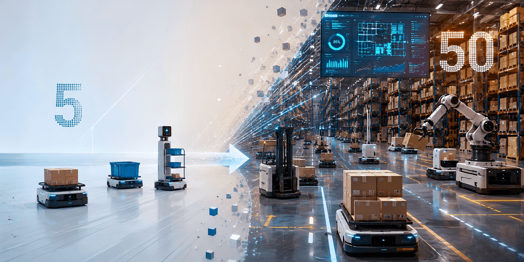
Scaling From 5 Robots to 50: What Breaks When Your Fleet Grows
What breaks when a warehouse robot fleet grows from 5 to 50, and the traffic, charging, network, and integration checks to complete before you expand.